Hi OpenCN developer,
After reading the documentation I understand that algorithm is implemented with Matlab and then converted to C++ code for real-time computation. But I’m not sure which Matlab script should I start from to run a trajectory planning example? And which script should I run to generate code for different platforms? Is there a workflow documentation for it or Could you give me some advice?
Hi,
one possibility is to run the script UnitTests.m in
matlab/common/UnitTests.m
The basic lines are :
cfg = FeedoptDefaultConfig;
cfg.source = ‘your_file.ngc’;
ctx = InitFeedoptPlan(cfg);
ctx = FeedoptPlanRun(ctx);
The scipt for generating C code is
generate_c.m
BUT : for the moment only possible with Matlab R2020a
We are working on a solution
best regards,
Raoul
Hi Raoul,
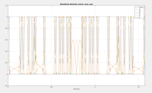
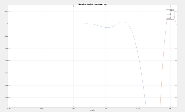
I found a script Validate_OpenCN.m. And after executing it and plot the planned results, I found some oscillations in the velocity file at the end or start of the ramp stage. Ideally it should be S curve? Will the fluctuation have an influence on the machining process?
From the documentation, the planning is optimization based. Do you have any reference about the planning method? Thanks!
Here is the velocity and position plot of the file spline_osc.ngc:
The velocity also vibrates. So is this a normal behavior of the current TP algorithm? I think ideally the velocity profile should be a 7-phase S curve.
There are many things to say :
The oscillations are of course unwanted.
They progressively disappear if the global parameters
NBreak and NDiscr are increased.
NBreak is the number of breakpoints for the spline q(u) used in Feedrate planning. NDiscr is the number of discretization points for the constraints.
Generally NDiscr should be roughly 2 times NBreak as a rule of thumb.
I believe the default values are NDiscr = 140 and NBreak = 60.
Spline support for compressing multiple small G01 segments is not yet fully operational in the master branch. It can be disactivated using parameter “Compressing” (file matlab/common/c_planner_v5/FeedoptDefaultConfig.m).
Improvements on the compressing feature are still in a separate branch which will be merged to the master soon.
1 Like
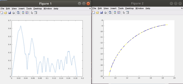
For a long straight line segment with stand still at both ends the optimal solution is of course a 7 phase trajectory where the accelaration has a trapezoidal shape :
rising, constant, falling, zero, falling, constant, rising
This was of course one of our first tests 
Please find enclosed a doc that also helps understanding the path planning.
PROCIR_HPC_2020_OpenCN_v6_revised.pdf (3.1 MB)
1 Like
Thank you Raoul! The paper is quite explainable. Only a few details I wish to understand further.
- Why the zero speed should be handled separately and the uk calculated in the following equation instead of Taylor series expansion? And what value should the constant pseudo jerk take?
- From Table 1, the number of knots for q(u) Nk is 10 but did not give the knot vector value {u0, u1, …, uk} and what is meaning of grid points for inequalities Ng?

- Why is too short or too long curves not preferred and they should be homogenized?
Hi yakunix,
-
There is a singularity at zero speed : if you use the Taylor series expansion you will stay at zero speed. Therefore the trick for using a constant pseudo jerk at the beginning. We implemented an algorithm for adapting the pseudo jerk in this phase of motion. We start with an initial value. If the constraints are violated we multiply the pseudo jerk by a factor < 1. This is repeated in a while loop until we find a pseudo jerk that does not violate the constraints. Even if it is not time optimal, this does not matter since it is only an extremely small part of the overall trajectory.
-
There are multiple knots at u=0 and u = 1. Refer to standard textbooks on B-Splines, eg. de Boor. Of course Nk (called NBreak in the code) is related to the number of basis functions of q(u).
The meaning of Ng (called NDiscr in the code) is the following : The constraints have to be respected for all real value of u in the interval [0, 1]. This means for infinitely many values. In order to convert it to a standard finite dimensional optimization problem, we only formulate the constraints on a finite grid of u values between 0 and 1. There is a technique called “spline relaxation” which can avoid this under certain conditions. I will explore this in a next release. I can send you publications on this topic. -
It is important that the optimization problems all have the same structure, same number of unknowns, same number of constraints, same sparsity structure. If NDiscr is fixed, the constraints for a long curve piece would be too rough. Discretizing extremely small curve pieces with the same NDiscr makes no sense since computation time will be too high. Homogenizing the length of curve pieces also helps to improving the conditioning of the optimization problems.
1 Like
Hi Raoul,
Thank you so much for the detailed information.
I spent some time reading the code and got some new doubts:
1.Could the zero speed singularity be handled by the following relation between t and u?
The question becomes: Given the time t, find the uk that satisfy the relation. We may use the bi-section method to search for the uk while for the integration, we may use Simpson or Gaussian integration method to approximate the result. Once we have got the solution uk for the first time tick (1e-4 in the code), then we are away from the singularity and then Taylor series expansion could be used.
2.The knot vector for q(u) is generated using the sinspace function. Is it a hypothesis for the optimization problem and what is motivation for using this type of knot vector?
3.In classic text book, the relation between number of control point ncoeff (n+1), number of knot vector nbreak (m+1) and degree of spline degree(p) is: m = n + p + 1, hence, ncoeff = nbreak - degree - 1. But in the code (bspline_create.m line 3), it is ncoeff = nbreak + degree - 2. I am not sure which one is right? Also, in the code, the spline degree is 4 rather than 3 in the paper, does it give a better result because typically higher degree would cause oscillations in the spline derivatives.
4.What are the meaning of the a_param, b_param, sp_index in the CurvStruct?
5.Could we simultaneously process the geometry smoothing and velocity planning? It seems as long as there are enough smoothed geometry in the queue, we can start to do the velocity planning. And could we start the motion once the first block in the horizon finished optimization?
Hi Yakunix,
I’m happy to have somebody asking good questions !
Welcome on board !
-
At zero speed you have a singularity in the integrand.
In the paper of Verscheure [VDS+09]
https://mecatronyx.gitlab.io/opencnc/opencn/CNC_Path_Planning_Algorithms/References/References.html
this singularity can be analytically solved if the unknown function q(u) is piecewise linear. However in order to have limited jerk this is not the case.
We spent a lot of time on the question how to handle this singularity, and the only solution we found is the idea to start with a constant pseude jerk. -
The choice of the knot vector can be either equidistant (linspace) or a higher density at the start and the end points. The function sinspace generates this non equidistant knot distribution. The idea behind was that changes in acceleration/deceleration are more likely to happen at the beginning and the end of each curve piece.
And the discretization scheme is more accurate if there is a higher density of knots.
Maybe it was not necessary. -
We played around with the spline degree; higher than 4 does not give any improvement. I’ll think about the other question.
-
The compressing yields a spline in R^3 which can be quite long.
The “splitting” homogenizes the length of of the curve pieces.
In order sto split, we introduce an affine function a_param*u + b_param on curve parameter u. If a_param = 1 and p_param = 0 you have the entire spline.
This means that several curve pieces can share the same spline coefficients.
sp_index is a “pointer” to the Spline coefficients which are not stored in the CurvStructs. -
YES, this is the idea. In fact the feedrate planning needs the most computation time.
Interpreting the .ngc file is extremely fast. The geometrical operations are also very fast.
No need to have parallel threads. However the feedrate optimization is really a parallel thread.
best regards,
Raoul
1 Like
Hi Raoul, thanks for your reply. It’s really helpful.
I think the variable SplineDegree in FeedoptDefaultConfig should be renamed to SplineOrder, because typically order = degree + 1. Or we can set SplineDegree = 3, and pass SplineDegree + 1 to gsl function.
1 Like
One more question… 
I noticed the equality constraints on the acceleration is enforced in its tangential component (with the projection operation). In this case, would the overall acceleration still be continuous considering the normal components?
It is sufficient to consider the equality constraint to enforce continuity of the tangential component, since the curvature at each junction point is continuous (G2 continuity).
Both components of the acceleration, normal and tangential will automaticall be continuous.
1 Like
That is Cool. Thanks!
Hi Raoul,
In the HPC paper, the remaining time is approximated by the following equation:
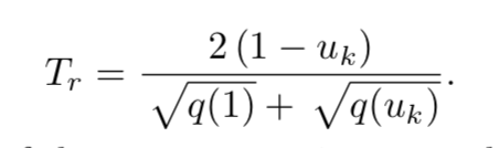
I’m wondering if this strategy could also be used for singularity handling. At the start of zero velocity, we can assume the q(u) to be linear, so we have the relation:
Then we have:
As q(uk) is a cubic spline and because q(0) is zero at start, we have q(u) to be the following format:
Substitute it into the denominator, we have:
This uk has a closed form of solution to be:
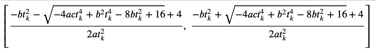
And we can choose the minimum positive solution.
Do you think the derivation is correct or did I mistake something?
Thanks!
hmmmm …
q(u) linear at the beginning will not work since the acceleration would jump which violates the jerk constraint.
In my memory we came to the conclusion that a cubic q(u) or even an arbitrary polynomial q(u) will not work in the beginning. There must be fractional powers in q(u).
It’s a long time ago, and I don’t remember all reasonings.
Okay… Sounds strange.
But when we formulate the problem, the constraint includes the initial boundary condition (v0 = 0, a0 = 0), right? In this case, the velocity and acceleration should be zero if we adopted the optimization results. Do you mean even if we uses the optimized q(u), the acceleration will still have a jump at the first cycle time? This will be contradictory since the solver thinks it has found a solution that will not violate the jerk constraint.
We can use very small tk like 1e-8 to solve the uk, and the spline q(u) will be almost linear at the infinite-small range . Once we have the first solution, then we are safe to use Taylor series expansion to get the remaining uk.
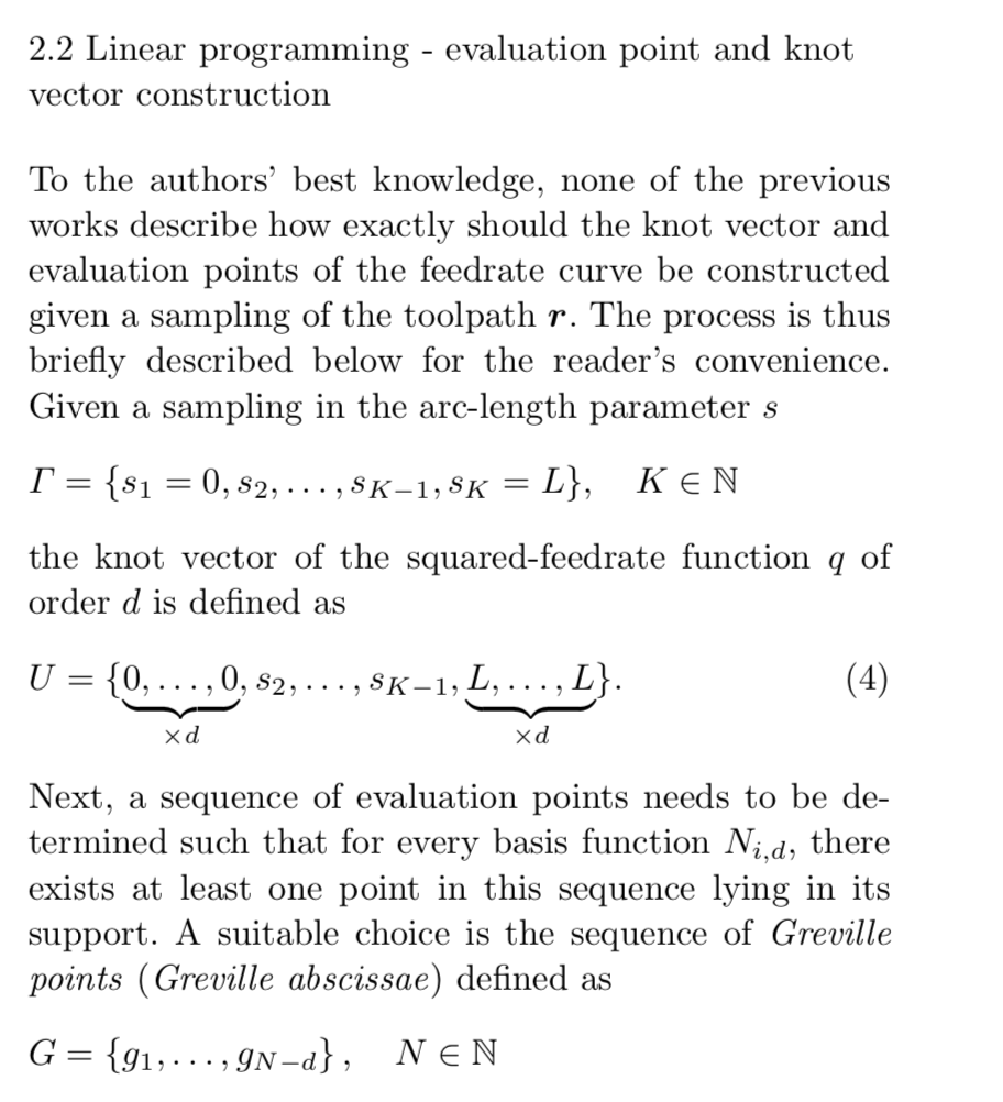
In the paper Linear programming feedrate optimization - Adaptive path sampling and feedrate override, it is mentioned that if we use the Greville abscissae as the evaluation sampling points, the optimization will be more stable since it results in a sparse M matrix. Current code uses a sinewave function to discretize the path. Maybe it is worth having a try.
thanks for your hint, that might be worth trying.
We started with an uniform knot distribution.
But acceleration/deceleration is likely to happen at the beginning and at the end of a curve piece. Therefore the “knot density” should be higher at the beginning and at the end. This leads us to use “sinspace” instead of linspace.
I never heard about Greville abscissae; I will have a look and come back to you later.
The wanted boundary conditions are indeed v0 = 0 and a0 = 0.
I will check with my mathematician friend Philippe Blanc next week and come back to you.
1 Like