Hi
One of the innovative features in OpenCN is our approach how smooth transitions between curve pieces are computed.
The approach is based on “Optimal Hermite” interpolation with geometric continuity G^2.
Refer to our publication
This initially only worked for curves in R^3.
But it turns out that it is quite simple to generalize our concept for curves in R^n.
This is work in progress and will be a cornerstone of our E2C project aiming at 5 axes support of OpenCN.
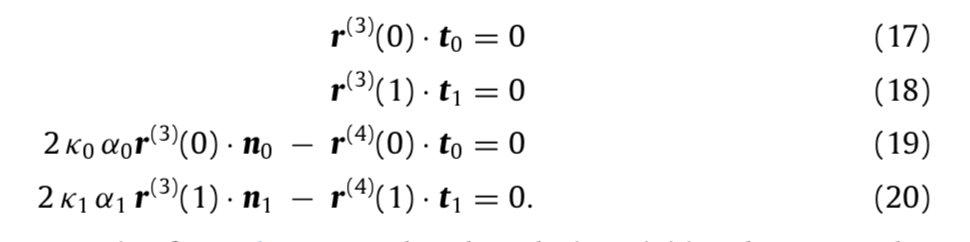
The generalization for the computation of transitions is based on the observation that the notion of curvature vector can be defined for curves in R^n without need of “cross product” in R^3.
We will introduce in the cost function a diagonal weighting matrix allowing to weight cartesian coordinates x, y, z against rotation angles, e.g. B and C.
The error between the programmed path (G code) and the transition is given by the distance between the “lift-off” points and the discontinuity point where the curve pieces intersect.
prepared by Philippe Blanc.
Il explains the generalization of the curvature vector in R^n, and the generalization of our approach for generating smooth transitions between curve pieces.
There will be a specific branch.
At my knowledge, the function
G2_Hermite_Interpolation.m
has already be changed for 5 axes.
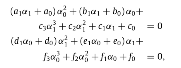
OK I see. So the coefficients of the polynomial system remains the same except the change of the calculation of the vector n.
I think it may also be useful for trajectory planning for manipulator in joint space R^n, where we have to create transitions between adjacent linear segments. Will give it a try.
Thanks!
Hi @Raoul, I found the transition creation has been updated in the opencn repo. But I did not find the matlab function to generate code from symbolic expression. For example, where is the symbolic expression for the function CoefPolySys? Thanks!
Our machine has a cartesian working space of ~50 x 50 x 50 mm.
The angles of the B and C axes are in degree, which is a comparable order of magnitiude. So the choice of our A matrix is identity.
We introduced A for future use where the cartesian and the rotary coordinates are not in a comparable order of magnitude.
Concerning the files for symbolic calculations, Hugo will reply you soon.
A “guide” for the choice of matrix A would be to choose a diagonal matrix with scaling factors enabling to scale all maximum excursions of cartesian and rotary coordinates to the normalized interval [-1, +1].
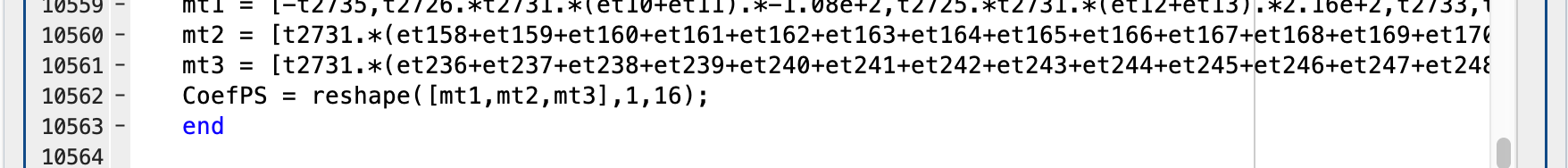
Thank you Raoul. I just modified the original symbolic script. It seems we can just remove the kappa param and resize the input vector. One thing I noticed is with the dimension increased from 3 to 5, the generated CoefPolySys.m will have more code (number of line increased from 257 to 1818). If I increased the dimension to 7, the generated file will have over 10000 line. Is it an expected behavior?
hi Yakunix,
in principle, the smooth transitions could be coded in such a way, that n is specified at run time and not in advance, and the number of Matlab lines would be independant on n.
Observe that a lot of scalar products between vectors occur in the calculations.
Unfortunately, the symbolic math toolbox breaks these scalar product up, i.e.
instead of x’ times y, you find x1 times y1+x2 times y2+x3 times y3+ etc etc
And during the symbolic calculations, the expressions become more and more complicated.
The Matlab symbolic toolbox is not able to handle symbolic vectors with unspecified size.
I see two possibilities :
doing the calculations by hand instead by the symbolic toolbox
with subs command, substitute scalar products by a new symbolic temporary variable
Our actual implementation is not elegant, I’ll check if there is a gitlab issue about this.
Thanks for pointing out this complexity issue.